Rendering the Mandelbrot set

Published 2025-12

Pictures based on the Mandelbrot set are a well-known staple of the pop-science Internet. I have always wanted to try my hand at generating them myself, so I finally sat down and did it.

The problem and its solutions are well-known, therefore I will not go into too much detail here. However, there are a few interesting implementation details that I found and that I would like to preserve. There are also a couple of open questions that I want to note down and maybe revisit in the future.

Problem statement

Just as a quick refresher, the Mandelbrot set is the set of \(c \in \mathbb{C}\) such that the sequence defined by \(z_0 = 0\) and \(z_{n+1} = z_n^2 + c\) does not diverge to infinity.

Mapping each pixel of an image to a specific value of \(c\), coloring each pixel that corresponds to a \(c\) in the Mandelbrot set black and each pixel that corresponds to a \(c\) not in the set a color based on how quickly the sequence diverges, we can generate interesting images.

A lot of pixels

Rendering this kind of image requires to do a bunch of calculations for each pixel. Fortunately each pixel is completely independent from the others, resulting in an embarrassingly parallel problem.

This seems like a perfect pretest to explore WebGPU, a modern graphics API exposed through web browsers and therefore available to websites. A very good introduction is available at WebGPU fundamentals.

The approach I decided to take is to use a vertex shader that renders a single rectangle covering the entire viewport, and a fragment shader that computes the color of each pixel.

A faster loop

The core of the algorithm, in pseudocode, is as follows:

z = complex(0, 0);
for i in 0..max_iterations {
    z = z * z + c;
    length = |z|;
    if length > 2 {
        break;
    }
}

This relies on the fact that \(\lVert z_n \rVert > 2 \ \rightarrow \ \lVert z_{n+1} \rVert > \lVert z_n \rVert \), which gives a condition that guarantees divergence and allows an early exit from the loop. The proof of this is well-known.

The first, trivial, optimization is to compare the squared length to 4, avoiding a square root operation.

A less trivial optimization requires expanding the operations on complex numbers:

z_re = 0;
z_im = 0;
for i in 0..max_iterations {
    z_re = z_re * z_re - z_im * z_im + c_re;
    z_im = z_re * z_im + z_im * z_re + c_im;
    length_sq = z_re * z_re + z_im * z_im;
    if length_sq > 4 {
        break;
    }
}

As shown in this article, the loop can be reduced from six multiplications and five additions to three multiplications and five additions per iteration:

z_re = 0;
z_im = 0;
z_re_squared = 0;
z_im_squared = 0;
for i in 0..max_iterations {
    z_im = z_re * z_im;
    z_im = z_im + z_im;
    z_im = z_im + c_im;

    z_re = z_re_squared - z_im_squared + c_re;
    z_re_squared = z_re * z_re;
    z_im_squared = z_im * z_im;

    length_sq = z_re_squared + z_im_squared;
    if length_sq > 4 {
        break;
    }
}

Colours!

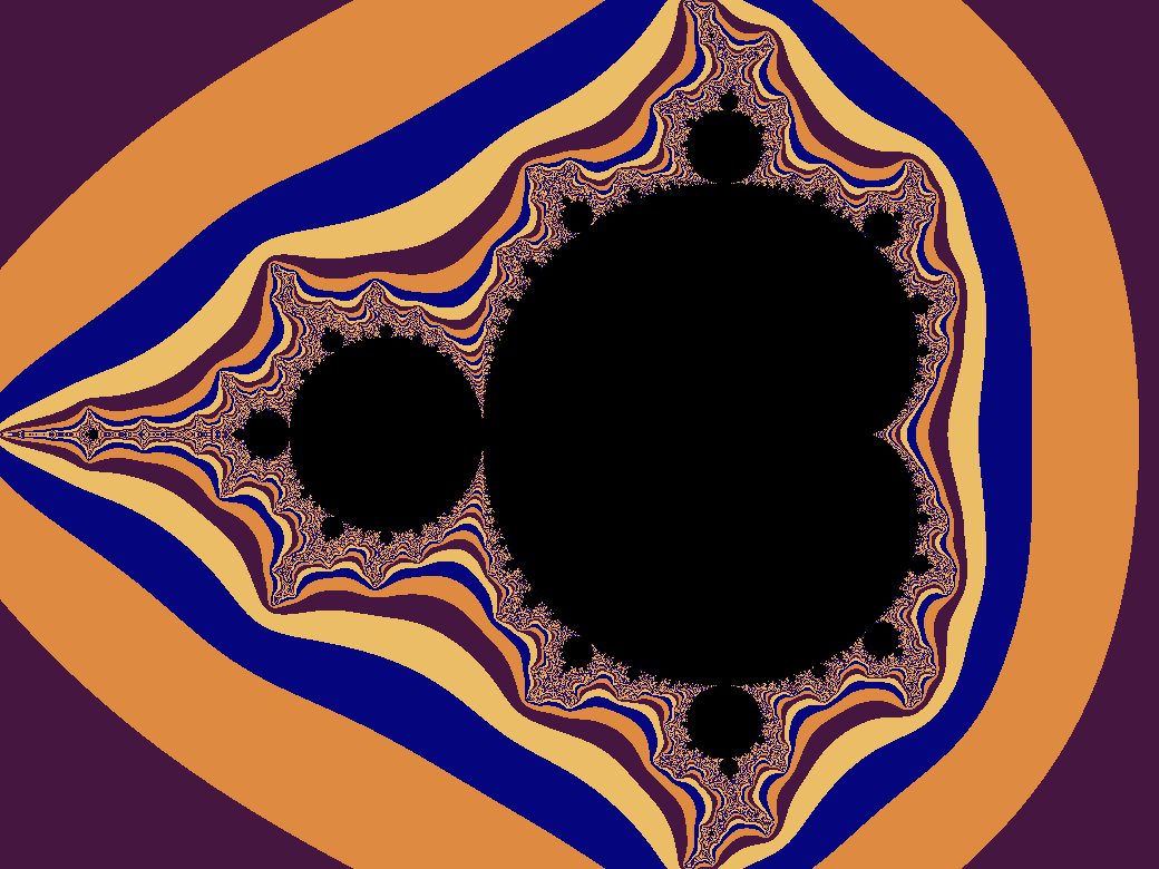
The colour of each pixel is determined by how quickly the sequence diverges. A simple approach uses directly the number of iterations before divergence to select a colour from a palette. However, since the number of iterations is an integer, this results in visible bands of colour:

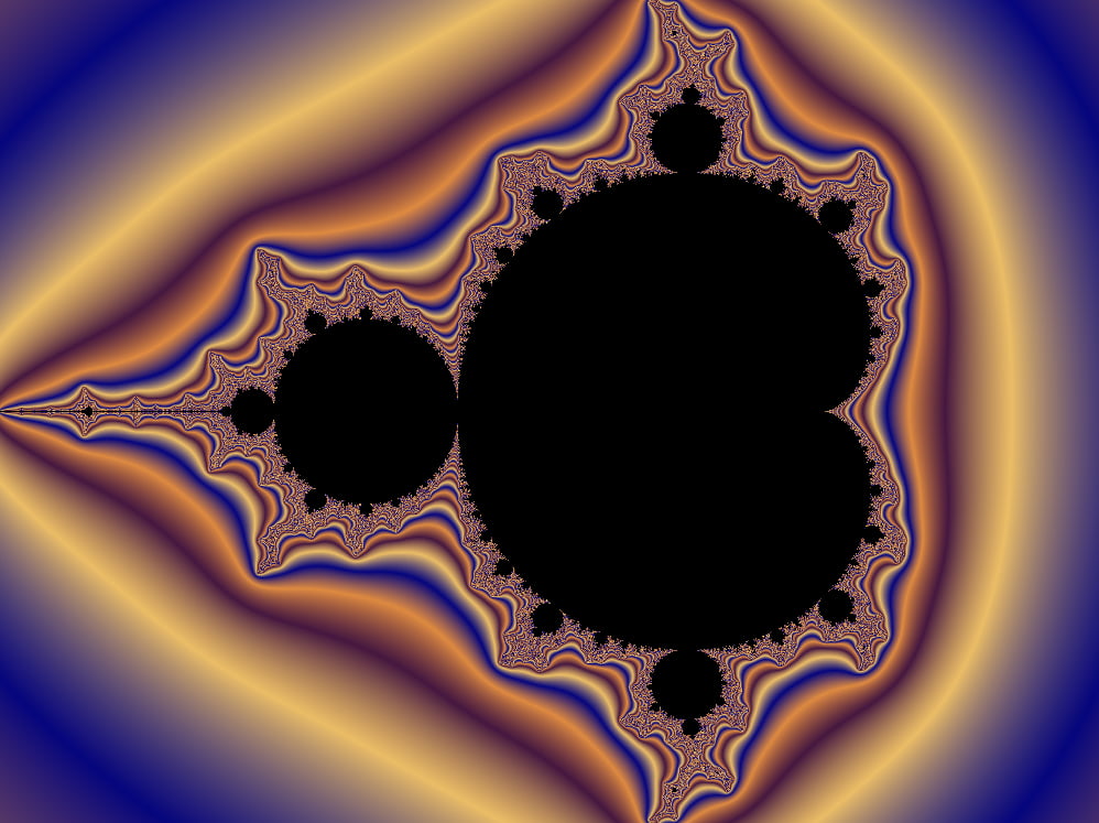
As explained in this article, there is a precise mathematical way to define a fractional iteration count, which can be used to generate smoothly-coloured images like the one at the beginning of this article.

Once again, reading the article I discovered an entirely new field of mathematics I never heard about, as I never had the opportunity to study complex analysis or holomorphic dynamics (see e.g. the video "Beyond the Mandelbrot set, an intro to holomorphic dynamics" from the 3Blue1Brow Youtube channel). Imagine getting started on a fun Christmas project and then end up reading a solution using "technique of spectral analysis of eigenvalues in Hilbert spaces".

Once again, I am surprised by where and how maths pops up, and by how unthinkable solutions follow almost naturally from the right mathematical framework. I never considered the idea of defining a fractional iteration count, but if you start thinking about a sequence as a repeated application of a function and you start wondering what means to apply a function \(\frac{1}{2}\) times, it flows quite naturally. This idea in turn can come from considering multiplication as a form of repeated addition and trying to use this framework to represent multiplications with fractional terms.

Regardless of the interconnectedness of mathematical knowledge and my limited view of it, I wanted to report here my understanding of the explanation given in the article, both to have it available and to keep it as a possible future learning topic. Errors in the transcription are mine.

The article introduces a function to compute this continuous iteration count, defined as follows:

\[ \mu(t) = \sum_{n=0}^{\infty} e^{-t \lVert f_n \rVert} \]

Where \(f_n\) is the \(n\)-th term of the sequence that defines the Mandelbrot set. The reasoning behind the choice of this specific function is beyond my current understanding. The article states that it is "analytically related to the Reimann Zeta-like regulator", but I wasn't able to reconstruct the reasoning behind it, or why it is relevant that for finite \(t\) and fast-enough growing \(f_n\) the sum \(\mu(t)\) converges.

The article then defines an escape radius \(R \in \mathbb{R}\) and an escape iteration count \(m\) such that:

\[ R < \lVert f_m \rVert \quad \land \quad \lVert f_{m+1} \rVert > R \]

The article then implicitly assumes that the desired fractional iteration count \(\mu_m\) is:

\[ \begin{eqnarray} \mu_m &=& \lim_{t \rightarrow 0^+}{\mu(t)} \\ &=& \lim_{t \rightarrow 0^+}{\left[\sum_{n=0}^{\infty} e^{-t \lVert f_n \rVert}\right]} \\ &=& \lim_{t \rightarrow 0^+}{\left[\sum_{n=0}^{m - 1} e^{-t \lVert f_n \rVert}\right]} + \lim_{t \rightarrow 0^+}{\left[\sum_{n=m}^{\infty} e^{-t \lVert f_n \rVert}\right]} \\ & \longrightarrow & x \in \mathbb{R} \land x \neq \infty \quad \Rightarrow \quad \lim_{t \rightarrow 0^+}{e^{-tx}} = 1 \\ & \longrightarrow & n \leq m - 1 \quad \Rightarrow \quad \lVert f_n \rVert \neq \infty \\ &=& m + \lim_{t \rightarrow 0^+}{\left[\sum_{n=m}^{\infty} e^{-t \lVert f_n \rVert}\right]} \\ &=& m + \lim_{t \rightarrow 0^+}{\left[\sum_{p=0}^{\infty} e^{-t \lVert f_{m + p} \rVert}\right]} \\ & \longrightarrow & p \in \mathbb{R}, \ p \geq m \quad f_{m+p} \approx f_{m}^{2^p} \quad \left(1\right)\\ &\approx& m + \lim_{t \rightarrow 0^+}{\left[\sum_{p=0}^{\infty} e^{-t \lVert f_{m}^{2^p} \rVert}\right]} \\ & \longrightarrow & \text{???} \\ &=& m + \lim_{t \rightarrow 0^+}{\left[\frac{\log(-\log(t))}{\log{2}} - \frac{\log(\log\left(\lVert f_m \rVert\right))}{\log{2}} + O(1)\right]} \\ & \longrightarrow & \text{"dropping the divergent terms"} \\ &=& m - \frac{\log(\log\left(\lVert f_m \rVert\right))}{\log{2}} + O(1) \\ &\approx& m - \frac{\log(\log\left(\lVert f_m \rVert\right))}{\log{2}} \\ \end{eqnarray} \]

Unfortunately, likely due to my lack of knowledge with the subject, I have not been able to reconstruct all the steps of the previous derivation. In particular, it is not clear to me how the author deduces that the sum of exponentials "diverges as \(\log(-\log(t))\) for small \(t\)" or why "dropping the divergent terms" is an allowed action.

The approximation at \((1)\) can be seen in the following by expanding the definition of \(f_n\):

\[ \begin{eqnarray} f_{n+p} &=& \underbrace{\left(\ldots \left(\left(f^2_n + c\right)^2 + c\right)^2\ldots\right)^2 + c}_{p \ \text{times}} \\ &=& O\left[\underbrace{\left(\ldots \left(\left(f^2_n\right)^2\right)^2\ldots\right)^2}_{p \ \text{times}}\right] = O\left[f_n^{2^p}\right] \approx f_n^{2^p} \\ \end{eqnarray} \]

Regardless of the questions that remain open, given a certain magnitude \(\lVert f_m \rVert\) of the iterated function just before the "escape", we are able to compute a fractional iteration count that can be used to smoothly interpolate between colours in a colour palette:

\[ \begin{eqnarray} \mu_n &=& m - \frac{\log(\log\left(\lVert f_m \rVert\right))}{\log{2}} \\ \end{eqnarray} \]

Numerical precision

One of the nice aspects of the Mandelbrot fractal is being able to zoom in a point and obtain very interesting visuals. This very quickly results in problems related to numerical precision.

This can be seen in the following image. They show the same section of the Mandelbrot set, but the left one is computed using 32bit of precision, while the right one uses 64bit:

64bit is still not sufficient for the very deep zoom animations, as those require up to ~1000+ bits of precision. This is a possible future extension for this project.